neural radiance fields (NeRF)

this project explores neural fields, specifically neural radiance fields (NeRF), as a method for representing 2d and 3d spaces. starting with a 2d example, we optimize a neural field to recreate an image, demonstrating the foundational concepts behind NeRF.

part 1: fit a neural field to a 2d image

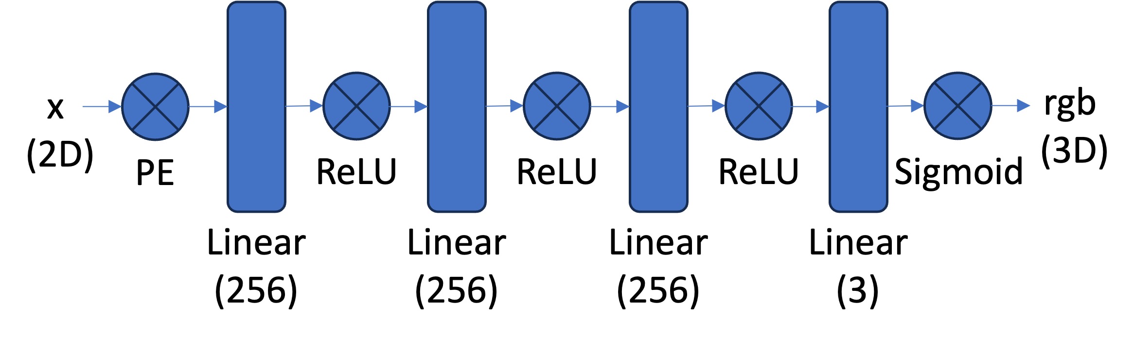
in this part, i implement a multilayer perceptron (MLP) network with sinusoidal positional encoding (PE), taking in 2-dim pixel coordinates and output the 3-dim pixel colors.

training settings:

model = MLP().to(device)
criterion = nn.MSELoss()
optimizer = optim.Adam(model.parameters(), lr=1e-2)
batch_size = im_w * im_h
iters = 3000

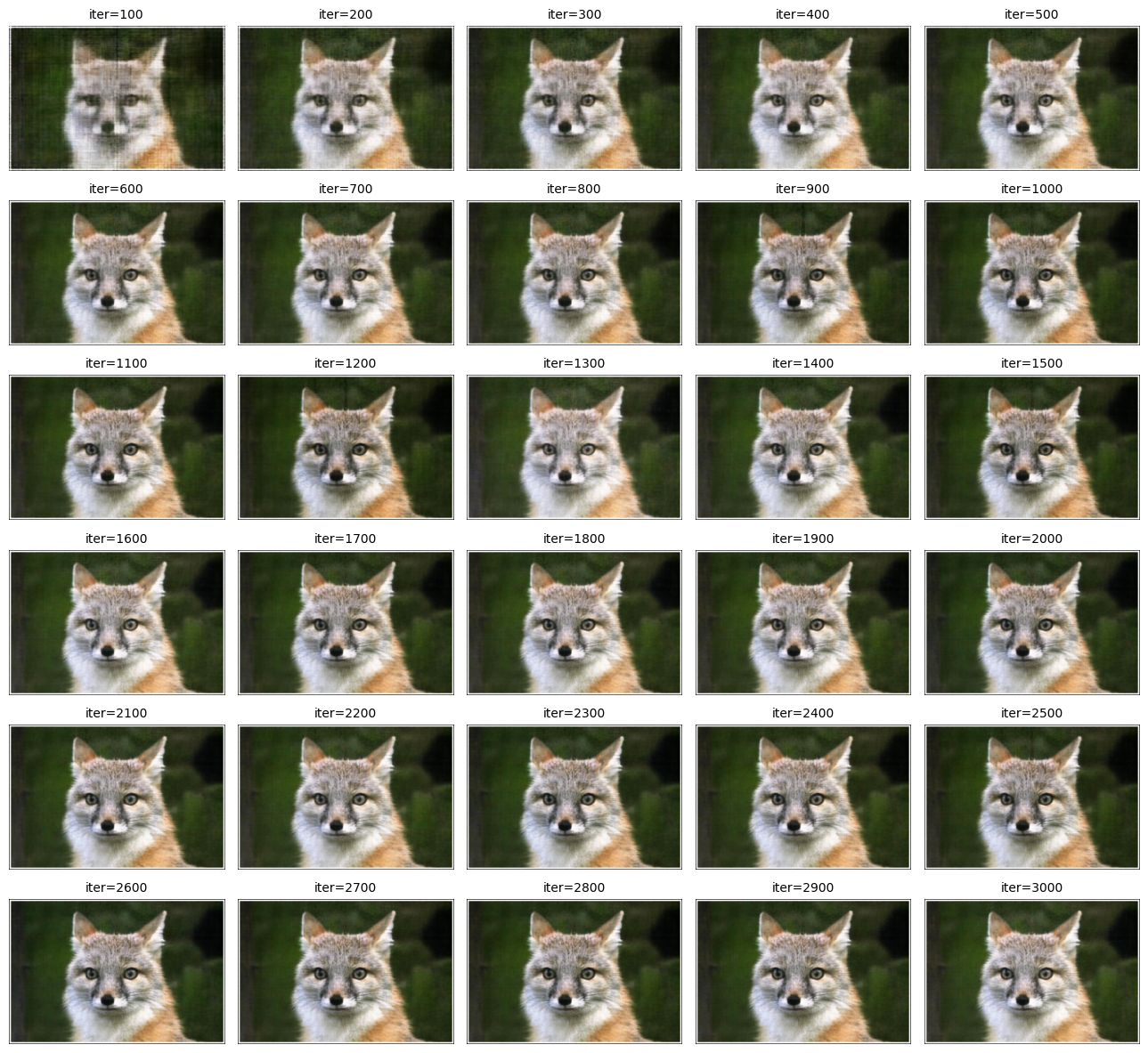
sample image 1: fox

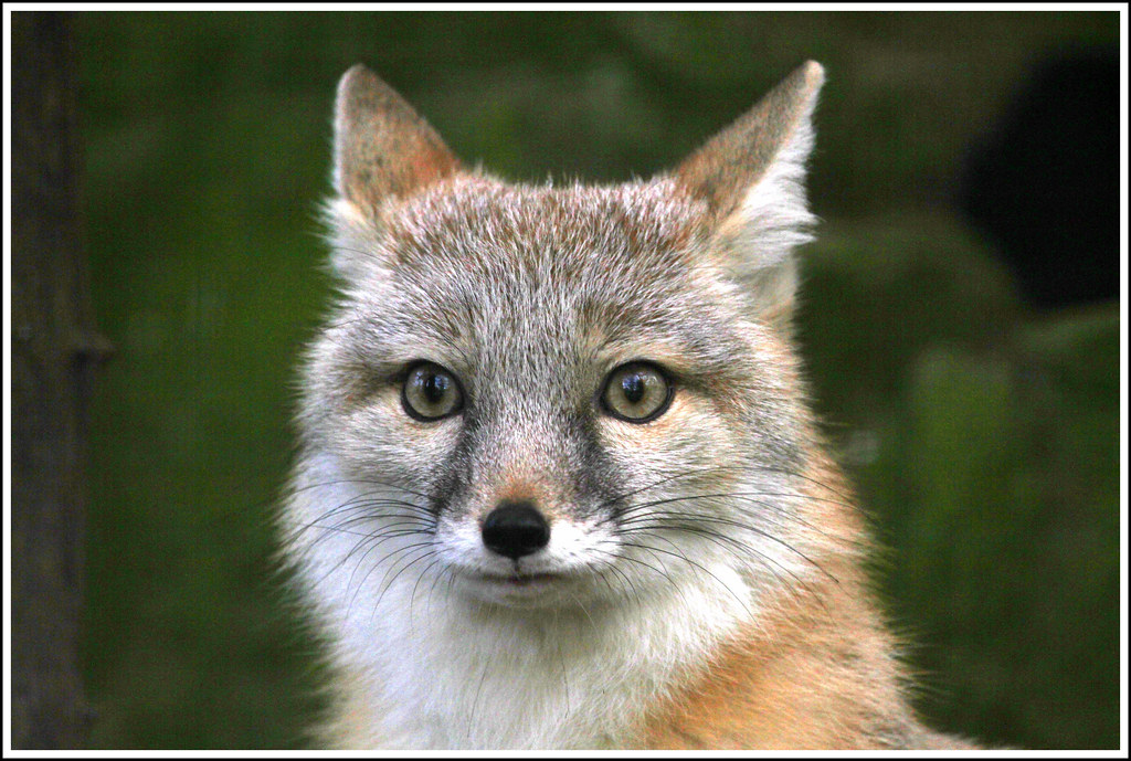
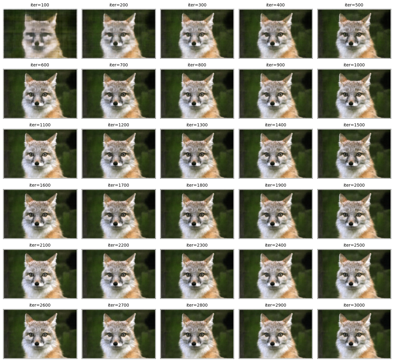
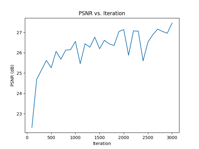
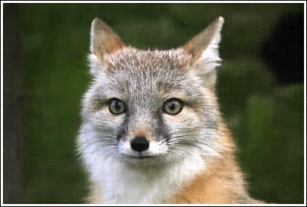
we can see that the final image generated by the mlp is a little darker than the original image. other than that, it looks pretty good!

sample image 2: langurs

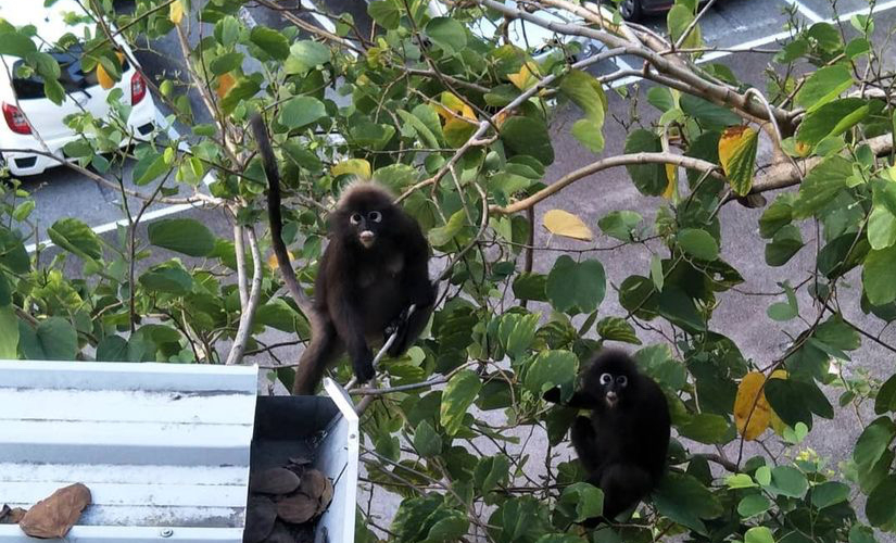
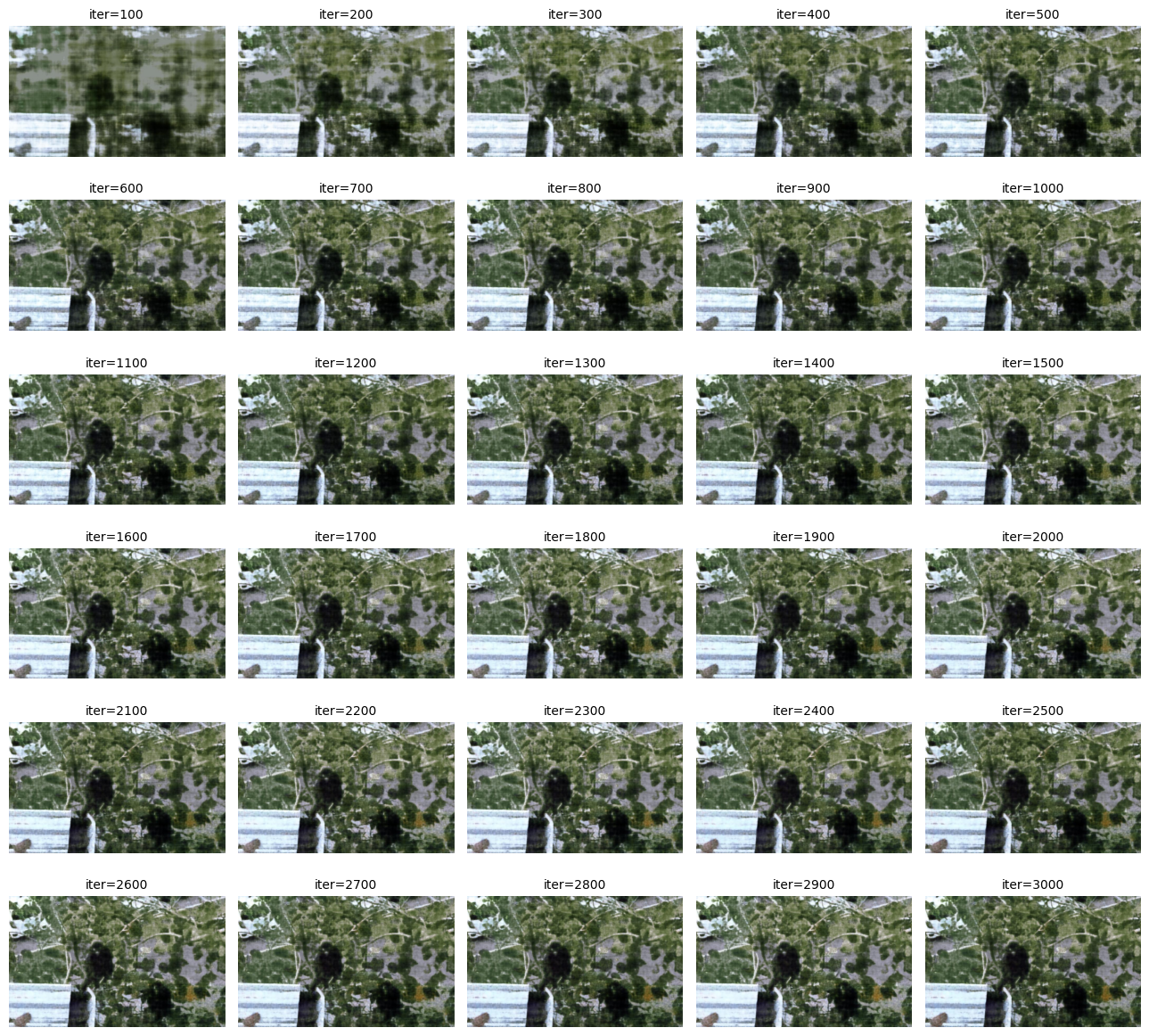
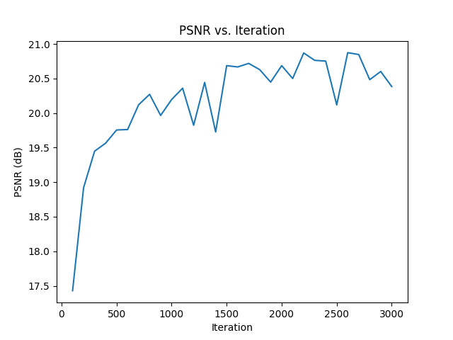
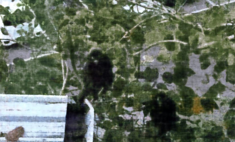
similar to the first image, the final image is darker than the original image. this image is slightly blurrier too. we can also see from our plot that the overall psnr is lower compared to the fox image. nonetheless, looks good.

hyperparameter tuning

let’s see if things change if we slightly alter the parameters. for this part i:

1. remove a fully connected layer + relu
2. change parameter L=10 to L=6

we see that the results are essentially the same! not much has changed.

part 2: fit a neural field from multi-view images

through inverse rendering from multi-view calibrated images, we can represent 3d space using a neural radiance field. we will be using the lego scene from the original NeRF paper

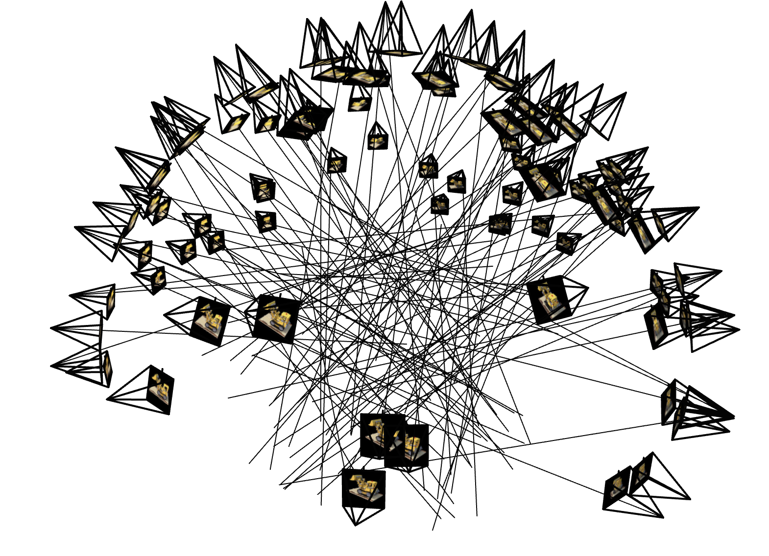
create rays from cameras

camera to world coordinate conversion

the transform function converts camera coordinates x_c to homogeneous coordinates by appending 1. using torch.matmul, these coordinates are batch-multiplied by the camera-to-world matrix c2w. the results are normalized by the last coordinate w.

pixel to camera coordinate conversion

the pixel_to_camera function reshapes and converts input u, v pixel coordinates into homogeneous coordinates. the camera intrinsic matrix k is inverted with torch.inverse and used to map the homogeneous pixel coordinates to camera coordinates. the result is scaled by the input depth s to produce x_c.

pixel to ray conversion

the pixel_to_ray function computes the world-to-camera matrix w2c as the inverse of c2w. from w2c, rotation r_inv and translation t are extracted to compute ray origins r_o = -r_inv * t. to calculate ray directions r_d, pixel-to-camera and camera-to-world transformations are applied, and the normalized vector difference x_w - r_o is computed.

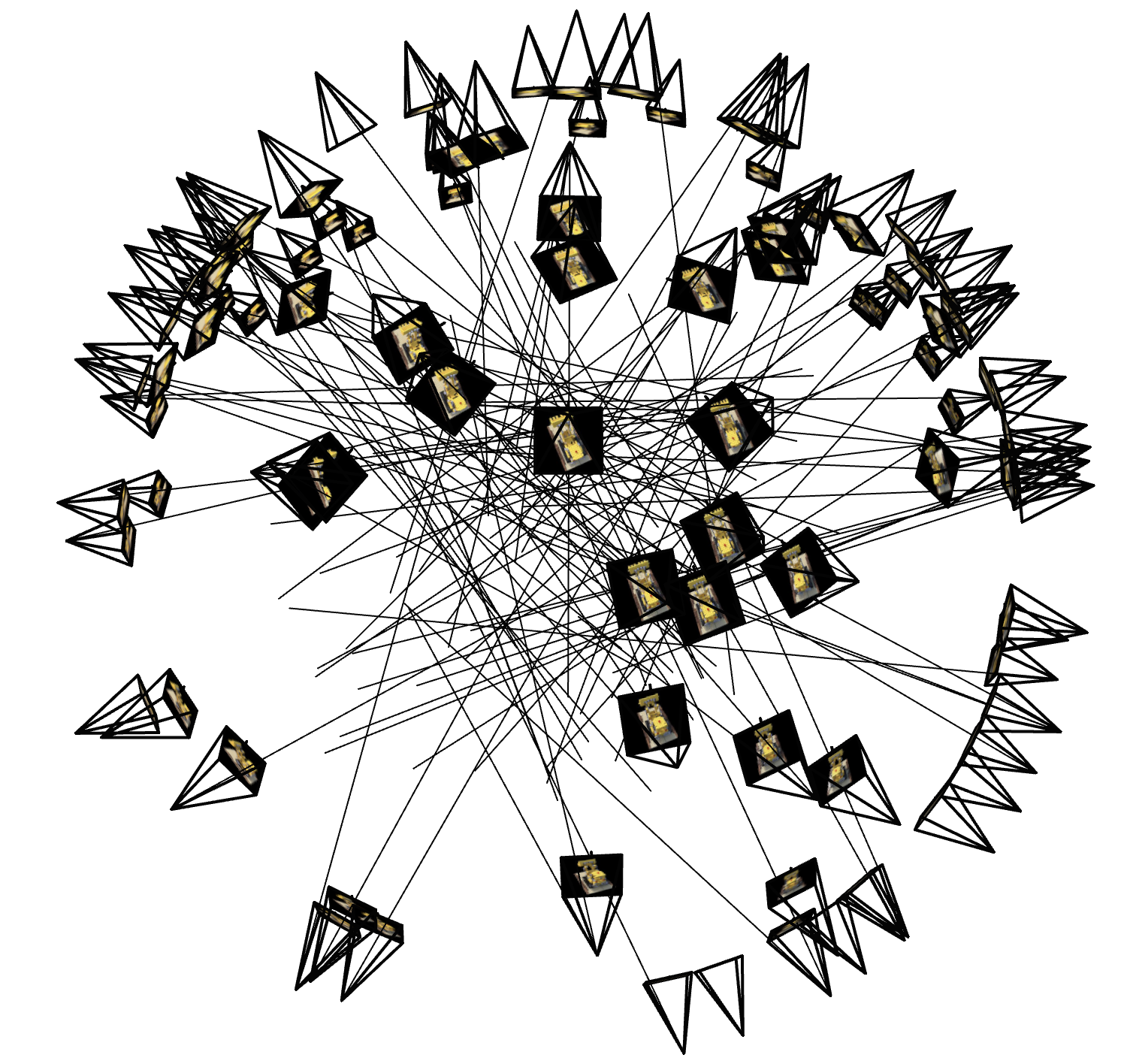
sampling

sampling rays from images

to sample rays from images, i flattened all the pixels from all the images and performed global sampling to get n rays from all images. i created a torch dataset called RaysData to hold these sampling functions. i included a function sample_rays which takes the number of rays n as an input parameter. i made sure to add 0.5 to all the uv coordinates so they sit in the center of the pixels. i call pixel_to_ray on my sampled uv values to get the sampled r_o and r_d.

sampling points along rays

i also implemented a function samples_along_rays which takes r_o and r_d as input. it also has metadata parameters including n_samples=32, near=2.0, far=6.0, and perturb=True. in this function, i uniformly create samples along the ray (stored in t). if perturb is true, i perturb the samples by a random amount. finally, i compute the final samples according to the formula x = r_o + r_d * t.

putting the dataloading together

i used the provided code (with adjustments) to make sure everything looked good.

neural radiance field

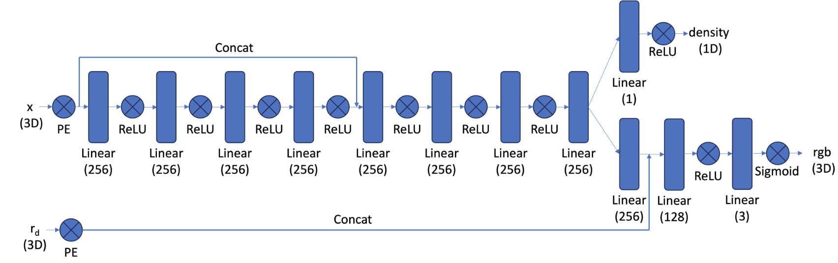
i implemented a multilayer perceptron (mlp) to predict both the density and color of 3d points in the radiance field. the network takes 3d world coordinates and view directions as input, applies positional encoding, and uses a deeper architecture with mid-layer concatenation to effectively optimize the 3d representation. i followed the following architecture:

training settings:

model = MLP().to(device)
optimizer = optim.Adam(model.parameters(), lr=1e-3)
criterion = nn.MSELoss()
batch_size = 10000
iters = 3000

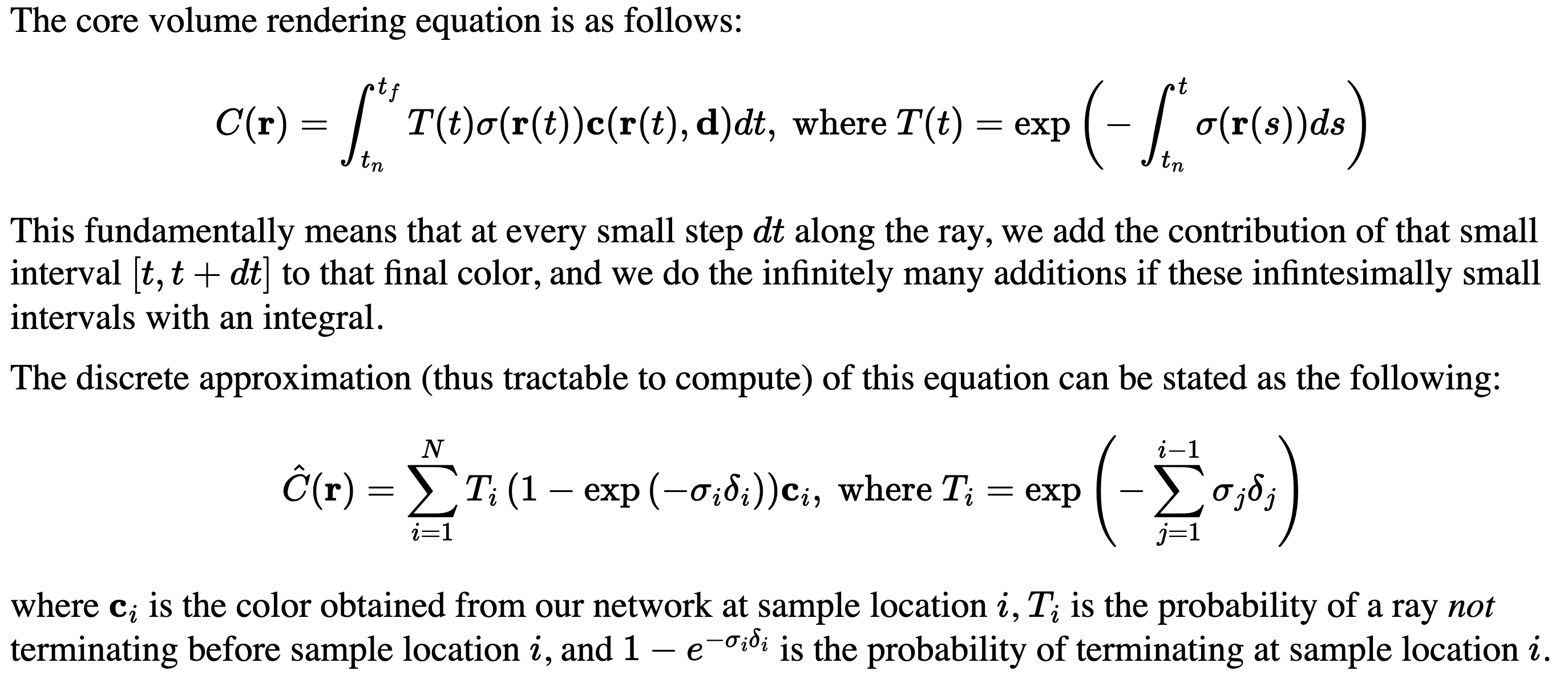
i implemented the volume rendering equation to compute the final color of rays by integrating over the density and color predicted by the network. the process involves calculating the transmittance along the ray, the opacity at each sample, and accumulating the color contributions from each sample. using pytorch, the implementation supports backpropagation by leveraging operations like torch.cumsum and torch.cumprod. this allows the network to be optimized end-to-end for tasks like novel view synthesis and depth estimation.

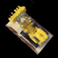
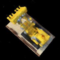
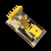
results

here are images of novel views from c2w_val generated by the nerf, with different numbers of epochs. to render an image from a single camera view, ray origins and ray directions are calculated for each pixel in the camera view.